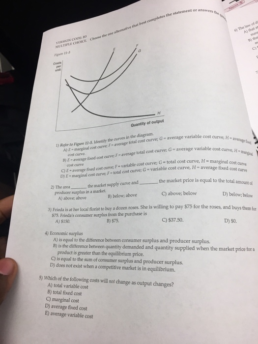
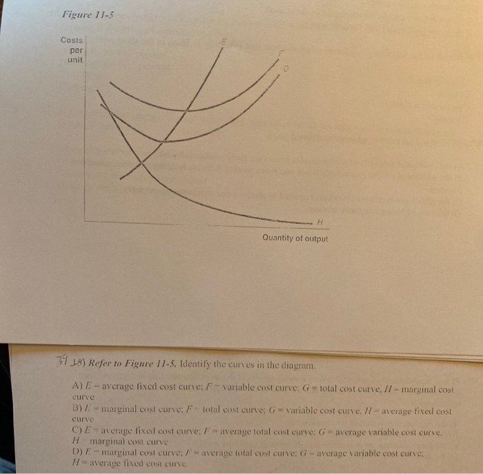
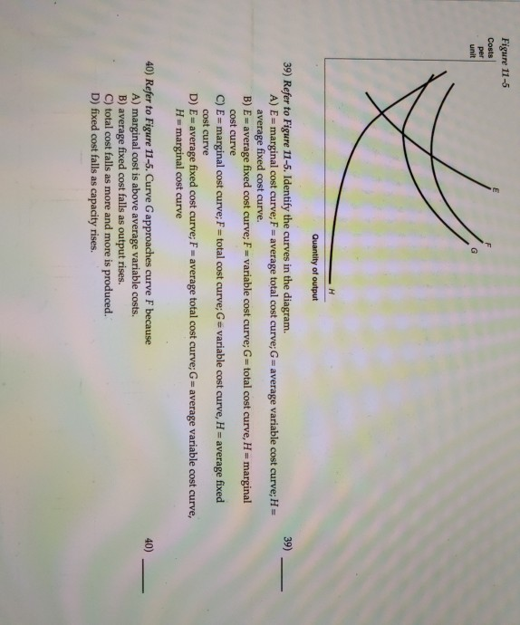
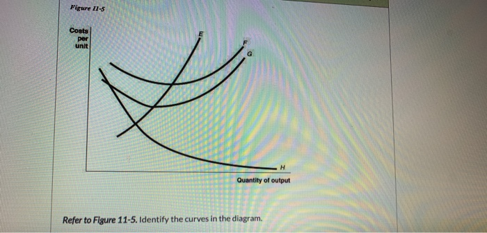
39 refer to figure 11-5. identify the curves in the diagram.
Solved Refer to Figure 11-5, Identify the curves in the | Chegg ... Question: Refer to Figure 11-5, Identify the curves in the diagram. A) E = marginal cost curves F = average total cost curve; G = average variable cost ...1 answer · Top answer: (1) (A) Since ATC = AVC + AFC, the ATC curve is above the other two c... 11.3 The Expenditure-Output (or Keynesian Cross) Model ... Figure 11.14 Equilibrium in the Keynesian Cross Diagram If output was above the equilibrium level, at H, then the real output is greater than the aggregate expenditure in the economy. This pattern cannot hold, because it would mean that goods are produced but piling up unsold.
PDF Answers to Phase Diagram Worksheet - Livingston Public Schools Refer to the phase diagram below when answering the questions on the back of this worksheet: NOTE: "Norma/' refers to STP — Standard Temperature and Pressure. 2.00 1.75 1.50 1.25 1.00 0.75 0.50 0.25 0.00 Temperature (degrees C) 1) What are the values for temperature and pressure at STP? T= 2) What is the normal freezing point of this substance?
Refer to figure 11-5. identify the curves in the diagram.
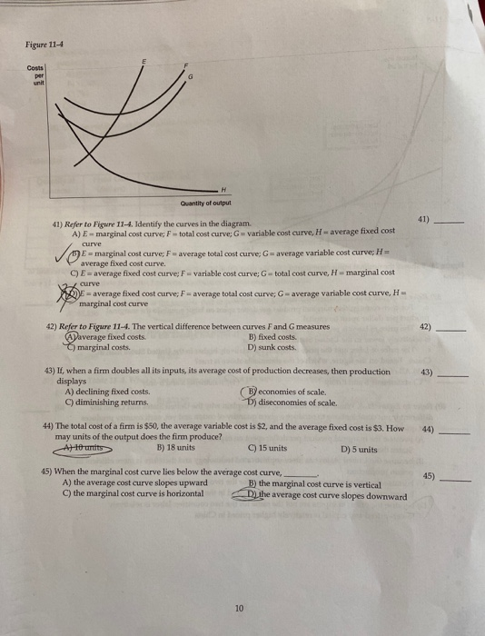
PDF Spring 2016 ECN1A Problem Set 4 Dr. Charles Liao Figure 11 -4 7) Refer to Figure 11 -4. What happens to the average fixed cost of production when the firm increases ... In a diagram showing the average total cost and average variable cost curves, the minimum point ... Figure 12 -5 Figure 12 - 5 shows cost and demand curves facing a typical firm in a constant - cost, perfectly competitive ... Solved Figure 11-5 Costs per unit н Quantity of output ... Transcribed image text: Figure 11-5 Costs per unit н Quantity of output Refer to Figure 11-5. Identify the curves in the diagram. E-marginal cost curve; F total cost curve; variable cost curve, H = average fixed cost curve E average fixed cost curve; F = average total cost curve: G average variable cost curve, H = marginal cost curve E marginal cost curve; F = average total cost curve; G ... PDF Module 4 Electronic Diagrams and Schematics - Energy Engineering Symbology, Prints, & Drawings Electronic Diagrams & Schematics 1 . OBJECTIVES TERMINAL OBJECTIVE 1.0 Given a block diagram, print, or schematic, IDENTIFY the basic component symbols as presented in this module.
Refer to figure 11-5. identify the curves in the diagram.. Figures (graphs and images) - APA 7th Referencing Style ... A figure may be a chart, a graph, a photograph, a drawing, or any other illustration or nontextual depiction. Any type of illustration or image other than a table is referred to as a figure. Figure Components. Number: The figure number (e.g., Figure 1) appears above the figure in bold. Title: The figure title appears one double-spaced line below the figure number in Italic Title Case. Microeconomics Flashcards | Quizlet Refer to Figure 11-5. Identify the curves in the diagram. ... Refer to Figure 11-5. Curve G approaches curve F because. average fixed cost falls as output rises. If the marginal cost curve is below the average variable cost curve, then. average variable cost is decreasing. Average fixed cost is equal to. Refer to Figure 11-5. Identify the curves in the diagram ... Refer to Figure 11-5. Identify the curves in the diagram. A) E = average fixed cost curve; F = average total cost curve; G = average variable cost curve, H = marginal cost curve. B) E = marginal cost curve; F = total cost curve; G = variable cost curve, H = average fixed cost curve. C) E = average fixed cost curve; F = variable cost curve; G ... ECON 3630 Test 3 Flashcards - Quizlet Refer to Figure 11-5. Identify the curves in the diagram. ... Refer to Figure 11-5. The vertical difference between curves F and G measures. average fixed costs. 1. If average total cost is $50 and average fixed cost is $15 when output is 20 units, then the firm's total variable cost at that level of output is.
DOC Nonprice competition refers to: - Weebly Assume Long Run for graphs A, B, and D. Identify the following market structures to answer questions 1-5 below: 1. Refer to the above figures. We would expect industry entry and exit to be relatively easy in: A) Figure A. B) Figure C. C) Figure B. D) Figures B and D. E) Figures A and C. 2. Refer to the above figures. Economics - Homework 7 Flashcards - Quizlet Figure 11-7 Figure 11-7 shows the cost structure for a firm. Refer to Figure 11-7. When the output level is 100 units average fixed cost is A. $10. B. $8. C. $5. D. This cannot be determined from the diagram. 36 Refer to Figure 12 9 Identify the firms ... - Course Hero Figure 12-17 The graphs in Figure 12-17 represent the perfectly competitive market demand and supply curves for the apple industry and demand and cost curves for a typical firm in the industry. 37) Refer to Figure 12-17. Which of the following statements is true? 37) A) The current market price is $3 but the price will increase in the future as the market demand increases. 42 refer to figure 11-5. identify the curves in the ... Refer to Figure 11-5. Identify the curves in the diagram. ... Refer to Figure 11-5. Curve G approaches curve F because. average fixed cost falls as output rises. If the marginal cost curve is below the average variable cost curve, then. average variable cost is decreasing. Average fixed cost is equal to.
Refer to Figure 11 5 Identify the curves in the diagram A ... Refer to figure 11 5 identify the curves in the. This preview shows page 5 - 8 out of 10 pages. A ) firms produce at the minimum point of their average cost curves . A ) average variable cost is minimized in production . B ) price must equal marginal revenue of the last unit sold . 11.2 Ohm's Law | Electric circuits | Siyavula 11.2 Ohm's Law (ESBQ6) Interactive Exercise 11.2. Try the interactive questions. Three quantities which are fundamental to electric circuits are current, voltage (potential difference) and resistance. To recap: Electrical current, I, is defined as the rate of flow of charge through a circuit. Potential difference or voltage, V, is the amount of ... 10.4 Phase Diagrams - Chemistry - opentextbc.ca Consider the phase diagram for carbon dioxide shown in Figure 5 as another example. The solid-liquid curve exhibits a positive slope, indicating that the melting point for CO 2 increases with pressure as it does for most substances (water being a notable exception as described previously). Notice that the triple point is well above 1 atm, indicating that carbon dioxide cannot exist as a liquid ... 11.7 Phase Diagrams - lardbucket In contrast to the phase diagram of water, the phase diagram of CO 2 (Figure 11.24 "The Phase Diagram of Carbon Dioxide") has a more typical melting curve, sloping up and to the right. The triple point is −56.6°C and 5.11 atm, which means that liquid CO 2 cannot exist at pressures lower than 5.11 atm.
Solved Figure 11-4 Costs - H Quantity of output 41) Refer to ...
Question 28 1 1 pts Figure 2 14 Refer to Figure 2 14 ... Question 28 1 / 1 pts Figure 2-14. Refer to Figure 2-14. Identify the two arrows in the diagram that depict the following transaction: Dorian Gray hires "Wild Oscar," a professional portrait artist, to paint his picture. J and Correct! K and G K and J and M M G. Question 29 1 / 1 pts Figure 2-14.

The Annual Cycle of SST in the Eastern Tropical Pacific ...
PDF Interpreting Phase Diagrams - uh.edu the two curves that descend towards the middle of the diagram from the melting points. These are the two liquidus curves. A liquidus curve separates a field of a single liquid from a field in which a solid and a liquid coexist in equilibrium. The first step in analyzing a phase diagram is to label the fields.
Metals | Free Full-Text | Fatigue Improvement of AlSi10Mg ...
19 Refer to Table 11 7 What is the marginal cost per unit ... Figure 11-7 Figure 11-7 shows the cost structure for a firm. 23) Refer to Figure 11-7. When the output level is 100 units average fixed cost is 23) A) $10. B) $8. C) $5. D) This cannot be determined from the diagram.
OSA | Athermal silicon photonic wavemeter for broadband and ...
(PDF) Long-run and Short-run Cost Curves - Academia.edu 2 The long-run cost curves, usually presented in a separate diagram, are also expressed most commonly in their average, or per unit, form, represented here in Figure 2. The long-run average cost (LRAC) curve is shown to be an envelope of the short-run average cost (SRAC) curves, lying everywhere below or tangent to the short-run curves.

Distinguishing shadows from surface boundaries using local ...
Pfd Calculus - measured points and predicted curves ed qp ... Pfd Calculus - 9 images - precalculus cleveland state university, ,
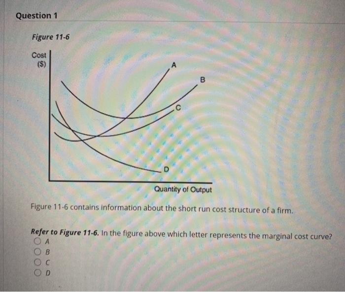
Solved Question 1 Figure 11-6 Cost ($) B Quantity of Output ...
Refer to Figure 12 9 At price P 1 the firm would produce A ... 12.5 "If Everyone Can Do It, You Can't Make Money at It": The Entry and Exit of Firms in the Long Run Figure 12-11 2) Refer to Figure 12-11. Suppose the prevailing price is $20 and the firm is currently producing 1,350 units. In the long-run equilibrium, the firm represented in the diagram A) will continue to produce the same quantity.
Heavy-fermion quantum criticality and destruction of the ...
Principles of Micro HW 7 Flashcards - Quizlet Refer to Figure 11-5. Identify the curves in the diagram. -E = marginal cost curve; F = total cost curve; G = variable cost curve, H = average fixed cost curve
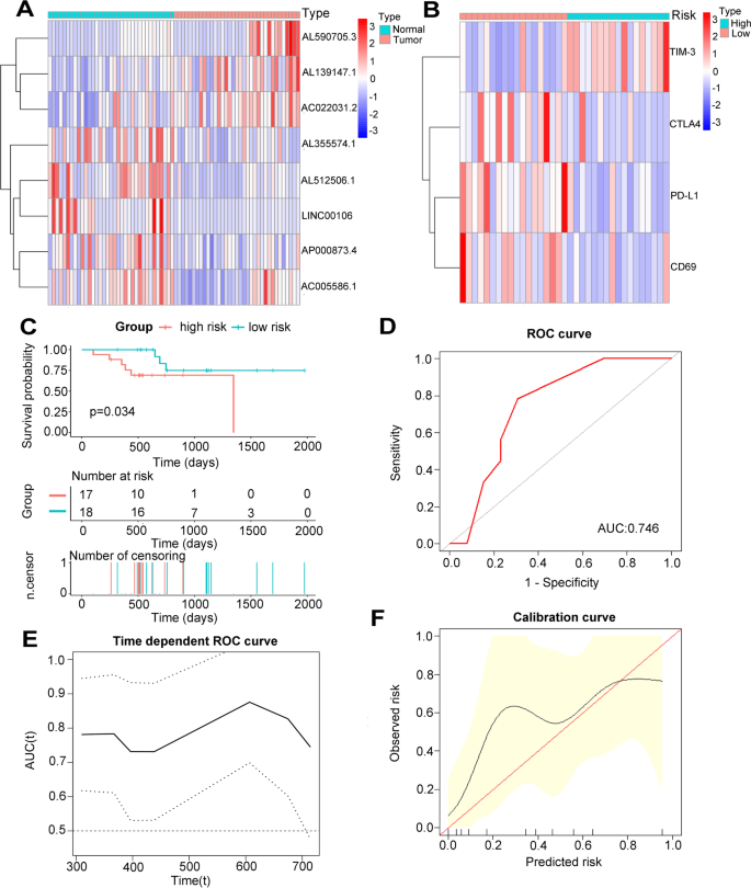
Comprehensive analysis of tumor immune microenvironment and ...
eco 11 Flashcards - Quizlet Refer to Figure 11-5. Curve G approaches curve F because a)total cost falls as more and more is produced. b)marginal cost is above average variable costs c)fixed cost falls as capacity rises. d)average fixed cost falls as output rises. d. Refer to Figure 11-5. Identify the curves in the diagram. a)E = marginal cost curve; F = total cost curve ...
![Solved] Figure 11-5 -Refer to Figure 11-5. Identify the ...](https://d2lvgg3v3hfg70.cloudfront.net/TB4188/11ea892a_4d60_c2ea_8f98_a36cbb84ce5f_TB4188_00_TB4188_00_TB4188_00.jpg)
Solved] Figure 11-5 -Refer to Figure 11-5. Identify the ...
PDF Module 4 Electronic Diagrams and Schematics - Energy Engineering Symbology, Prints, & Drawings Electronic Diagrams & Schematics 1 . OBJECTIVES TERMINAL OBJECTIVE 1.0 Given a block diagram, print, or schematic, IDENTIFY the basic component symbols as presented in this module.

Quenching and Distortion*
Solved Figure 11-5 Costs per unit н Quantity of output ... Transcribed image text: Figure 11-5 Costs per unit н Quantity of output Refer to Figure 11-5. Identify the curves in the diagram. E-marginal cost curve; F total cost curve; variable cost curve, H = average fixed cost curve E average fixed cost curve; F = average total cost curve: G average variable cost curve, H = marginal cost curve E marginal cost curve; F = average total cost curve; G ...
Mean-field analysis of orientation selectivity in inhibition ...
PDF Spring 2016 ECN1A Problem Set 4 Dr. Charles Liao Figure 11 -4 7) Refer to Figure 11 -4. What happens to the average fixed cost of production when the firm increases ... In a diagram showing the average total cost and average variable cost curves, the minimum point ... Figure 12 -5 Figure 12 - 5 shows cost and demand curves facing a typical firm in a constant - cost, perfectly competitive ...
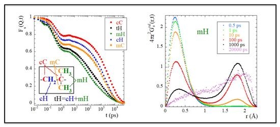
Polymers | Free Full-Text | Disentangling Self-Atomic Motions ...
An investigation into the deep learning approach in ...
Solved Figure 11-5 Costs per unit G H Quantity of output ...

Distinguishing shadows from surface boundaries using local ...

Chapter 11 Flashcards | Quizlet
Crystals | Free Full-Text | Influence of Crystal Plasticity ...
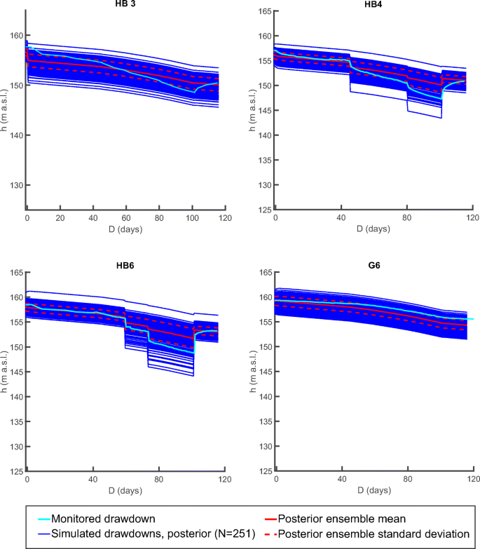
Ensemble-based stochastic permeability and flow simulation of ...
Solved Refer to Figure 11-5, Identify the curves in the ...

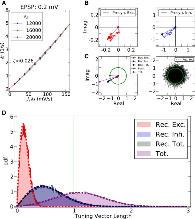
Local and collective transitions in sparsely-interacting ...

Qualitative aspects of Rastall gravity with barotropic fluid

Acquired resistance to anti-MAPK targeted therapy confers an ...
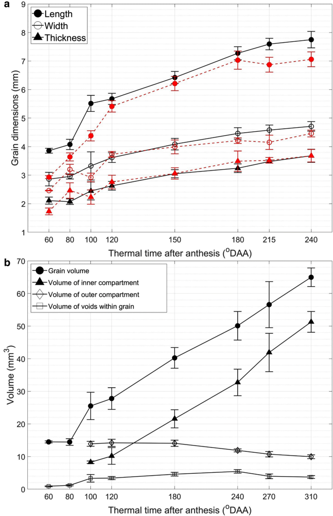
Use of X-ray micro computed tomography imaging to analyze the ...
Solved Figure 15-2 Price and cost per unit P MC ATO PS LATC₂ ...

On the thermal coarsening and transformation of nanoscale ...
Dynamics of resonant x-ray and Auger scattering
Anchor-free network with guided attention for ship detection ...

Measurement Potential of the Barkhausen Effect for Obtaining ...
An efficient Equilibrium Optimizer for parameters ...
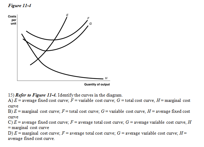
Solved Refer to Figure 11-4. Identify the curves in the ...

Plane Parallel Albedo Biases from Satellite Observations ...
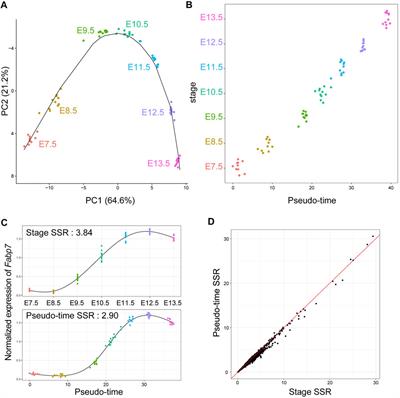
Frontiers | Intracellular and Intercellular Gene Regulatory ...
Solved Of Figure 11-1 Total Produet 15 8 Labor (units) 36 ...

The BEST framework for the search for the QCD critical point ...
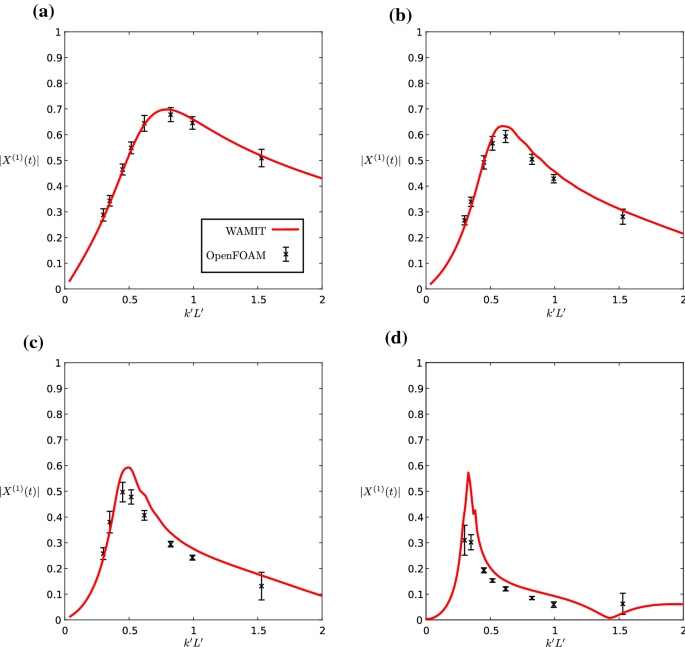
Numerical analysis of wave–structure interaction of regular ...
Solved Figure 11-5 Costs Quantity of output Refer to Figure ...

The Coevolution of Massive Quiescent Galaxies and Their Dark ...
Remote Sensing | Free Full-Text | Climate Data Records from ...

Measurement Potential of the Barkhausen Effect for Obtaining ...
0 Response to "39 refer to figure 11-5. identify the curves in the diagram."
Post a Comment